Well log interpretation that stays on your machine
A browser-based petrophysics workspace for loading LAS and DLIS well logs, running Vsh through net pay in structured views, and staging zone averages for Volumetrics, without uploading your log files or saved cases to our servers.
Included on the Starter plan and above. Formation Evaluation projects save to a folder you choose on your computer; they do not count toward Starter’s cloud saved-case limit. See Starter pricing
Formation Evaluation saves projects to a folder you choose on your computer using the File System Access API: case JSON, LAS files, trend lines, and display templates live in that project folder. We do not store well log files or interpretation cases in Supabase, and no log format is uploaded to parse: LAS, ASCII, LIS (binary LIS 79 included) and DLIS are all read in the browser. When you bridge zone results to Volumetrics, the handoff stays in your browser (local module bridge). CSV import elsewhere on the platform follows the same browser-only pattern where enabled.
Confidentiality with the operator
Petrophysicists working under operator confidentiality terms often cannot send raw logs to third-party cloud storage. This module is designed so interpretation work remains on the device you control; sharing is manual (export project package or case files) when you choose to involve a teammate.
Workspace views
Each case moves through dedicated views (same order as the in-app View menu):
Log viewer: load LAS 1.2 to 3.0 or RP66 V1 DLIS (pick the frame and logical file), alias curves, QC, and apply display templates
Vsh workspace: shale volume from GR, SP, neutron–density, and related indicators
Porosity workspace: density, neutron, sonic, and combined models with shale endpoints
Sw workspace: 7 saturation model families (Archie, Simandoux, Modified Simandoux, Indonesia, dual-water, Waxman-Smits, and Juhasz)
Net pay workspace: cutoffs, coal handling, and net/gross flags
Results and sensitivity: zone tables, exports, and cutoff sensitivity
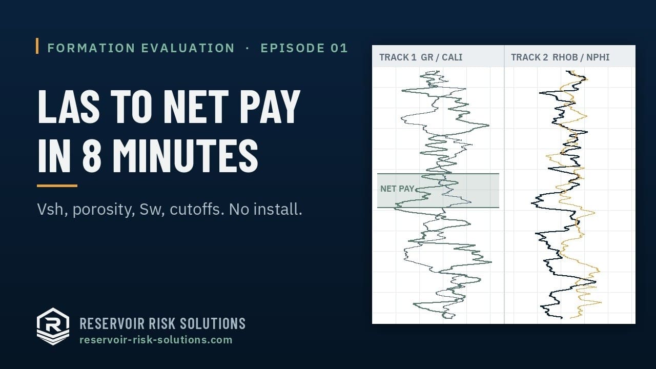
The sample well RRS‑SYN‑0001, from LAS file to net pay (7:55).
Also in the workspace
Beside the seven views, the workspace carries the field, production and export tools a study needs, all reading the same case:
Batch interpretation: the same route across every case in the project in one run, with one parameter set or each case's own, outlier QC flags, a posted base map, and exports for all the wells at once
NMR: the T2 distribution partitioned into bound and free fluid (BVI and FFI) at a sandstone, carbonate or custom cut-off, irreducible Sw, and Coates permeability
Production: Arps exponential, hyperbolic and harmonic decline fits on imported history, and gas p/z material balance that extrapolates to gas in place
Core: routine-core-analysis corrections before calibration, Klinkenberg gas slippage with the Heid slip factor and overburden-stress multipliers, then core-to-log calibration plots
Export: LAS 2.0, LAS 3.0 with core, tops, perforation, test and survey sections, RP66 V1 DLIS, CSV, an Excel workbook, a per-well ZIP, and a true-scale log PDF (1:200, 1:240 and others) with the zone summary
Offline: after one visit while signed in, the workspace opens without a connection on a signed pass, for up to 7 days or 100 hours of offline use, whichever comes first; interpretation, exports and the project folder all work, while billing and cloud saves wait for the network
Beyond the seven core views, the Compute menu adds specialist interpretation you would normally leave the workspace for. Every mode reads the same curves, depth reference, zones, alias table, and unit system as the rest of your case, and writes results back as depth curves you can plot, cross-plot, and export.
Porosity and lithology
Neutron–density crossplot porosity
Apparent porosity from neutron–density crossplot tie lines, using the NPHI calibration already set in your interpretation parameters. No display template needed; the calibration follows the case.
Methods: Crossplot tie-line solution with matrix and fluid end-points
Neutron–sonic crossplot porosity
Apparent porosity from neutron–sonic tie lines for intervals where the density log is washed out, missing, or affected by barite mud.
Methods: Crossplot tie-line solution with NPHI calibration and fluid transit time
Neutron matrix conversion
Convert a raw neutron curve recorded on one matrix to the matrix you are interpreting on, so limestone-scaled and sandstone-scaled logs across a field can finally be compared.
Methods: Standard neutron matrix correction table, calibration lithology from interpretation parameters
Fuzzy lithology classification
Classify sandstone, limestone, dolomite, and shale from a curve suite without hand-drawing cut-offs on every crossplot. Output is a class-code curve you can carry into net pay and zone work.
Methods: Fuzzy c-means clustering of gamma ray, neutron, density, and resistivity
Multimineral solver
Probabilistic multimineral inversion, the second interpretation route beside the deterministic Vsh, porosity and Sw workspaces: it solves component volumes from your log end-points under physical constraints (every volume at or above zero, all volumes summing to one) rather than letting an unconstrained fit return mineral fractions that cannot exist.
Methods: Tool-uncertainty-weighted constrained least-squares inversion from user-defined log end-points, optional Monte Carlo on the end-points
Permeability
Permeability from logs
Estimate permeability from effective porosity and water saturation using the published transform that matches your rock, with the choice visible in the case rather than buried in a spreadsheet formula.
Methods: Timur, Tixier, Wyllie–Rose, Kozeny–Carman, and Coates free-fluid transforms
Neural network permeability
Where a published transform does not fit the rock, train a small network on your own core calibration points and predict permeability from porosity plus up to three further log curves.
Methods: Feed-forward neural network trained on your core plug data
Rock typing
Rock typing and hydraulic flow units
Split the core porosity–permeability cloud into populations that each obey their own transform, then predict which one every log sample belongs to. A single global k–φ transform is usually the largest error in a computed permeability curve; two plugs at the same porosity can differ by two orders of magnitude in permeability, and one regression through the whole cloud is wrong for both. Each rock type carries its own fitted transform, its own average k and φ for a saturation-height model, and a published class name where the method has one.
Methods: Amaefule RQI/FZI flow units, Winland R35 port size, Lucia rock-fabric number, silhouette-scored clustering, and a Gaussian classifier that reports its own confidence
Saturation and pressure
Saturation-height modelling
Model water saturation from height above the free water level instead of from resistivity, the independent check that matters in thin beds, low-resistivity pay, and wells where the resistivity answer is disputed.
Methods: Power-law, Swirr-anchored, and Leverett J-function forms built from capillary pressure and k/φ
Formation pressure analysis
Import RFT and MDT pressure points, fit gas, oil, and water gradients, and read fluid contacts straight off the gradient intersections rather than inferring them from logs alone.
Methods: Gradient fitting with GOC, OWC, and FWL from gradient intersections
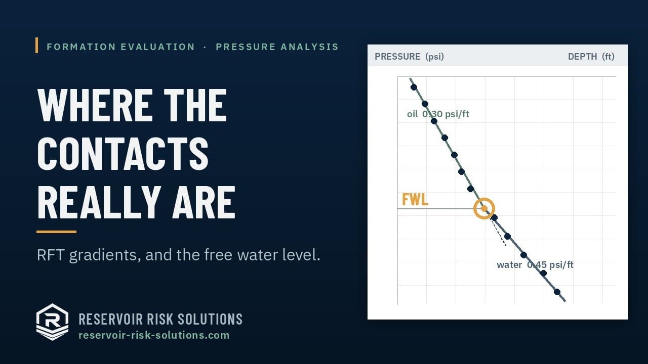
Gradients fitted to the RRS‑SYN‑0001 pressure stations, and the free water level they give (8:51).
Geomechanics
Geomechanics (1D mechanical earth model)
A full wellbore stability model along the well: elastic properties with shear synthesis, overburden, pore pressure, rock strength, poroelastic horizontal stresses, the safe mud weight window, a stress polygon, sanding onset pressure, and brittleness (Rickman elastic from the model's own moduli, mineralogical from solver volumes), calibrated against imported RFT/MDT and LOT/FIT points.
Methods: Eaton and Bowers pore pressure, McNally / Horsrud / Golubev UCS, Kirsch hoop stresses with Mohr–Coulomb failure, Rickman elastic and Jarvie / Wang–Gale mineralogical brittleness
Organic matter (TOC and kerogen) as a step of the interpretation
Total organic carbon and kerogen volume for source rocks and unconventional plays, computed as the step between shale volume and porosity so it is part of the interpretation rather than a bolt-on: the ΔlogR baselines are the shale points you already picked for Vsh, the porosity models subtract the kerogen from the matrix on every log, net pay gains a TOC cut-off, and the zone table, uncertainty and Volumetrics bridge carry the TOC. Calibrate to core and carry the answer forward with its uncertainty. Every method is discounted where it is known to fail: the ΔlogR overlays in gas zones, tight carbonates and over-mature rock, the density method in bad hole, so the fused curve comes with a per-depth confidence and a reason flag instead of one method's silent bias. Kerogen is then subtracted from the matrix in the porosity workspace, the zone table reports organic-rich thickness, TOC·h and Langmuir adsorbed plus free gas in place with richness classes, and the bridge carries the adsorbed gas content into Volumetrics.
Methods: Passey ΔlogR (sonic, density and neutron overlays with LOM from Ro or Tmax), Schmoker density–kerogen volume, uranium regression, validity-weighted fusion with confidence, core TOC calibration, parameter Monte Carlo P10–P90, Langmuir isotherm gas content with temperature and ash corrections
Tie the well to seismic from sonic and density: acoustic impedance, integrated two-way time, normal-incidence reflectivity, and a convolved synthetic trace, without exporting curves to a separate geophysics package.
Methods: Acoustic impedance, time–depth integration, and Ricker wavelet convolution
Crossplots
Custom crossplot
Cross-plot any two curves the well carries, logged or calculated, when the standard neutron–density, Pickett, and Hingle views do not frame the question you actually have. An axis can be committed back to the well as a depth curve, so a relationship you find on the plot becomes a curve the rest of the interpretation can use.
Methods: Arbitrary curve pairs with optional axis commit back to the well
Bridge to Volumetrics
When zone averages are ready, stage NTG, porosity, Sw, and net pay for the Volumetrics module through an explicit in-browser handoff. You review the payload before confirming; nothing is applied silently downstream.